HRV Analyzer

The HRV Analyzer calculates basic HRV (Heart Rate Variability) statistics for each epoch.

Table of contents

Introduction
User Corrections
HRV Analyses
Processing and Analysis Pipeline
Settings
Metrics
References

Introduction

The HRV Analyzer retrieves corrected IBI (Inter Beat Interval) data from a linked ECG module, detrends it, and performs epoch-based analyses to extract several time-domain, frequency-domain and non-linear HRV measures.

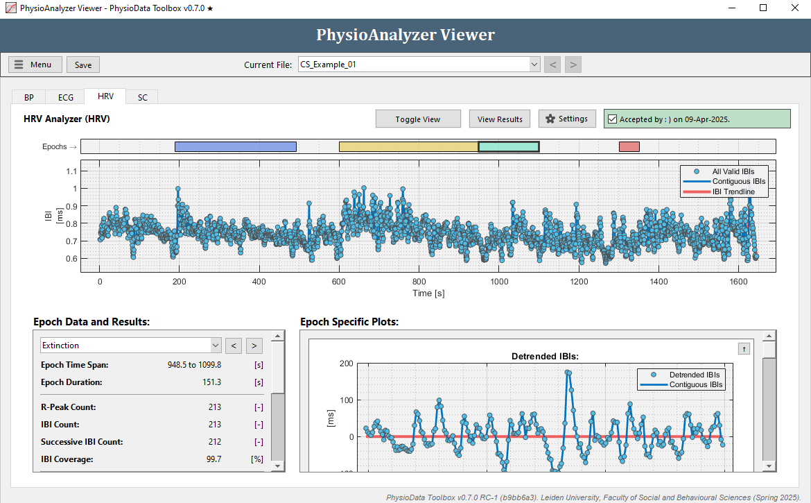
The two topmost graphs of the HRV module visualize the epochs, the IBI data that were retrieved from the ECG module and—if enabled—the global trend baseline. Below those are two panels labeled Epoch Data and Results and Epoch Specific Plots, which show the analysis results and plots of the selected epoch.

The time-domain, frequency-domain, and non-linear results are visualized for the current epoch in the GUI’s two bottom panels. Users can navigate to another epoch by selecting it from the dropdown menu in the Epoch Data and Results panel, or by clicking the buttons next to it. Additionally, epochs can be selected by clicking on the epoch rectangles in the epoch graph.

User Corrections

The HRV module itself does not allow users to correct artifacts, this must instead be done in the linked ECG module. Any changes made to the IBIs in the linked ECG module are automatically transmitted to the HRV module, and the graphs and results table are automatically updated.

HRV Analyses

The HRV module performs a collection of time-domain, frequency-domain and non-linear analyses on detrended IBIs located within a specific epoch. See the Metrics section for a full overview of the output.

Time-Domain Analysis

The HRV module extracts the following standard time-domain metrics from the detrended IBI data:

Percentage of absolute differences between successive IBIs that exceed 20 ms (pNN20) and 50 ms (pNN50).
IBI standard deviation.
Root Mean Squared of Successive Differences (RMSSD).

The RMSSD and the successive IBI differences from which it was calculated are visualized in the module’s Successive Differences graph in the Epoch Specific Plots panel.

Detrended IBIs and RMSSD — Figure 2: The detrended epoch-specific IBIs (top) and the differences between them (bottom). For visualization purposes, the heart rate acceleration events are plotted in pink and the heart rate deceleration events in aquamarine. Note that a heart rate acceleration is defined as an increase in heart rate, which equals a decrease in inter beat interval.

Frequency-Domain Analysis

The Lomb-Scargle method is used to estimate the IBI time-series’ Power Spectral Density (PSD), from which the Very Low Frequency (VLF), Low Frequency (LF), and High Frequency (HF) powers are computed.

Lomb-Scargle Periodogram — Figure 3: A Power Spectral Density estimate computed using the Lomb-Scargle periodogram method. The Very Low, Low and High Frequency bands are visualized in purple, red and green, respectively.

Non-Linear Analysis

The HRV module generates a Poincaré plot for the non-linear analysis of HRV. A Poincaré plot is a scatter plot where each IBI (IBI_n) is plotted against the subsequent IBI (IBI_n+1), with the former and latter representing the horizontal and vertical axes, respectively. The Poincaré plot refers to IBIn and IBIn+1 as RR_n and RR_n+1 in order to better comply with convention.

Processing and Analysis Pipeline

The data processing and analysis pipeline used by the HRV module is described below:

Step 1: IBI sourcing and Global Detrending

The corrected IBIs from the linked ECG module are retrieved. If enabled by the user, the IBI trend is then calculated by first resampling the IBIs at 4 Hz, and then using the smoothness priors approach ¹ and the user-specified lambda value to compute the trend baseline.

Lambda — Figure 5: The high-pass cutoff frequency of the smoothness priors detrending filter as a function of lambda (λ), as computed for a 10 minute epoch.

Step 2: Epoch Segmentation and Detrending

The epoch-specific IBIs are isolated by copying all IBIs and rejecting those located outside of the current epoch, with the ‘IBI location’ for a given IBI event being defined as the timestamp of the R-peak that ends that inter beat interval.

If smoothness priors detrending is enabled by the user, the epoch-specific IBIs are detrended by subtracting from each IBI its corresponding trend baseline value, as visualized by the red line in the IBI graphs. The epoch-specific IBIs are then also linearly detrended. This is done subsequent to the smoothness priors detrending, or in absence of it if that is disabled.

All subsequent steps are performed on the epoch-specific detrended IBIs unless otherwise specified.

Step 3: Calculating Time-Domain Metrics

First, the standard deviation of the IBIs is calculated, which gets reported as the IBI_std_detrended metric. Because the detrended IBIs are used, this standard deviation should be less than the standard deviation calculated by the ECG module, which uses the actual non-detrended IBIs.

Subsequently, the detrended IBIs that are ‘contiguous’—i.e., directly adjacent to each other—are identified and used to calculate the successive differences. The root mean squared of these differences is then calculated and reported as RMSSD_detrended. This metric is also calculated by the ECG Signal Analyzer module, but from the non-detrended IBIs. However, since RMSSD is not strongly influenced by slower IBI oscillations, the RMSSDs reported by both modules should not differ substantially.

Additionally, the fraction of absolute successive differences that exceed 20 and 50 ms are calculated and reported as a percentage in pNN20_detrended and pNN50_detrended respectively.

Step 4: Calculating Frequency-Domain Metrics

First, the PSD of the detrended IBI time-series is estimated using MATLAB’s implementation of the Lomb-Scargle periodogram and a frequency resolution of 0.0001 Hz. An error is thrown if the epoch does not feature enough IBIs to resolve the required frequency range. If enabled in the module’s settings, the PSD is then smoothed using a ‘loess’ filter and the specified span. Any negative PSD values that may result from the smoothing are set to 0.

The band powers are then calculated from the smoothed PSD for the following ranges, adjustable in the module’s settings:

Very Low Frequency (VLF):
0.0033 – 0.04 Hz.
Low Frequency (LF):
0.04 – 0.15 Hz.
High Frequency (HF):
0.15 – 0.4 Hz.

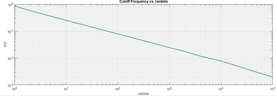
By default, the detrending lambda is set to 500, which equals an approximate high-pass cutoff frequency of 0.04 Hz given the resampling frequency of 4 Hz. This strongly attenuates the VLF power, so analyzing sub 0.04 Hz frequencies may require that either the smoothness priors detrending be disabled or that the lambda be increased.

The absolute powers are reported in ms² as the metric XF_power, where XF is either VLF, LF or HF. Additionally, the percentages of each power band as a fraction of the total power is reported in the XF_powerPercent metric.

For each of the VLF, LF, and HF bands, the highest peak is detected and its value and frequency are logged. These data are exported as XF_psdPeak and XF_psdPeakFreq, respectively. No data is exported for a certain band if that band does not contain a peak.

Step 5: Poincaré Analysis

To generate the Poincaré plot, all the epoch-specific IBIs that have a directly subsequent IBI are identified. These IBIs are labeled IBIn and their subsequent IBIs are labeled IBI_n+1. The Poincaré plot is then generated by plotting IBIn against IBI_n+1, with the former and latter representing the horizontal (X) and vertical (Y) axes, respectively.

A diagonal identity line (X = Y) is then generated, and the standard deviations of the Poincaré data-points is calculated in the direction of the identity line (SD2) and in the direction perpendicular to it (SD1). Depending on the module’s Poincaré plot IBI source setting, either the original IBIs or the detrended IBIs are used.

Settings

The HRV must be linked to an ECG module in order for it to function. This is done by filling in the tag of the ECG module in the Tag of the ECG Analyzer field.

The auto-generated list below shows the settings available in the HRV Analyzer module:

General Settings:
Name, source and epoch settings for this PhysioAnalyzer.
- Analyzer prefix (tag):
  The tag (name) of this PhysioAnalyzer. The tag must be unique and start with a letter, and may only contain alphanumeric characters.
- Tag of the ECG Analyzer:
  The tag of the ECG Analyzer from which the accepted IBIs are used.
- Generate epochs from:
  Specifies how epochs are generated.
Global Detrending Settings:
The IBI series can be detrended using the smoothing priors method, which can be enabled and configured using the settings below.
- Smoothing priors detrending [-]:
  The lambda for the smoothing priors detrending.
PSD Estimation Settings:
The Power Spectral Density is estimated using the Lomb-Scargle method, then divided into the Very Low, Low and High Frequency bands using the settings below.
- VLF power band [Hz]:
  The lower and upper limits of the Very Low Frequency band.
- LF power band [Hz]:
  The lower and upper limits of the Low Frequency band.
- HF power band [Hz]:
  The lower and upper limits of the High Frequency band.
- LS Periodogram smoothing [Hz]:
  The window size of the moving average smoothing filter applied to the LS periodogram.
Poincaré Plot Settings:
The Poincaré plot can be generated either from the original IBIs or from the detrended IBIs.
- Poincaré plot IBI source [ ]:
  The IBIs to use when generating the Poincaré plot.

Metrics

The auto-generated table below lists all the metrics produced by the HRV Analyzer module.

Table 1: The metrics calculated by the HRV Analyzer module.

Variable:	Unit:	Description:
timeDomain_error	-	Time-domain analysis errors.
RMSSD_detrended	ms	The Root Mean Squared of the Successive Differences between contiguous IBIs, as computed from the detrended IBIs.
IBI_std_detrended	ms	Standard Deviation of the accepted discrete IBI data points (SD normalized by (N-1), where N is the sample size), as computed from the detrended IBIs.
pNN20_detrended	%	Percentage of absolute differences between successive IBIs that are greater than 20 ms, as computed from the detrended IBIs.
pNN50_detrended	%	Percentage of absolute differences between successive IBIs that are greater than 50 ms, as computed from the detrended IBIs.
LS_error	-	Lomb-Scargle periodogram calculation errors.
VLF_powerPercent	%	The power of the Very Low Frequency band, calculated using the Lomb-Scargle method, as a percentage of the sum of the VLF, LF and HF powers.
VLF_power	ms^2	The absolute power of the Very Low Frequency band, as calculated using the Lomb-Scargle method.
VLF_psdPeak	s^2/Hz	The highest power spectral density peak in the Very Low Frequency band. Empty values may indicate that the band did not feature any peaks.
VLF_psdPeakFreq	Hz	The frequency at the highest power spectral density peak inside the Very Low Frequency band. Empty values may indicate that the band did not feature any peaks.
LF_powerPercent	%	The power of the Low Frequency band, calculated using the Lomb-Scargle method, as a percentage of the sum of the VLF, LF and HF powers.
LF_power	ms^2	The absolute power of the Low Frequency band, as calculated using the Lomb-Scargle method.
LF_psdPeak	s^2/Hz	The highest power spectral density peak in the Low Frequency band. Empty values may indicate that the band did not feature any peaks.
LF_psdPeakFreq	Hz	The frequency at the highest power spectral density peak inside the Low Frequency band. Empty values may indicate that the band did not feature any peaks.
HF_powerPercent	%	The power of the High Frequency band, calculated using the Lomb-Scargle method, as a percentage of the sum of the VLF, LF and HF powers.
HF_power	ms^2	The absolute power of the High Frequency band, as calculated using the Lomb-Scargle method.
HF_psdPeak	s^2/Hz	The highest power spectral density peak in the High Frequency band. Empty values may indicate that the band did not feature any peaks.
HF_psdPeakFreq	Hz	The frequency at the highest power spectral density peak inside the High Frequency band. Empty values may indicate that the band did not feature any peaks.
LF_HF_ratio	-	The Low Frequency power divided by the High Frequency power.
poincare_error	-	Poincare calculation errors.
poincare_SD1	ms	The poincare SD1: the standard deviation of RRn against RRn+1, in the direction perpendicular to the diagonal RRn = RRn+1 line.
poincare_SD2	ms	The poincare SD2: the standard deviation of RRn against RRn+1, in the direction of the diagonal RRn = RRn+1 line.
poincare_SD2_SD1_ratio	-	The poincare SD2 divided by the poincare SD1.
HR_mean	BPM	Mean of the continuous Heart Rate, as interpolated from the accepted IBI data points.
R_peakCount	count	Count of accepted R-peaks inside current epoch, including user-defined added R-peaks.
IBI_mean	s	Arithmetic mean of the accepted discrete IBIs. IBI values are defined as: IBI(n) = Rt(n)-Rt(n-1), and are timestamped using: IBIt(n) = Rt(n).
IBI_min	s	Min value of the accepted discrete IBI data points.
IBI_max	s	Max value of the accepted discrete IBI data points.
IBI_std	s	Standard Deviation of the accepted discrete IBI data points (SD normalized by (N-1), where N is the sample size).
IBI_count	count	Count of accepted IBI data points inside current epoch.
IBI_coverage	%	The percentage-wise IBI coverage of the epoch; i.e., 100*(sum of the IBIs)/(Epoch Duration).
HRV_ssdCount	count	Count of succesive IBIs inside current epoch. Nonadjacent IBIs are not considered succesive.

References

Tarvainen, M. P., Ranta-Aho, P. O., & Karjalainen, P. A. (2002). An advanced detrending method with application to HRV analysis. IEEE Transactions on Biomedical Engineering, 49, 172-175. doi: 10.1109/10.979357 ↩