Basic Walkthrough
The basic tutorial will teach users the core concepts of the Toolbox, and how to import, visualize, clean and analyze data.
Table of contents
Introduction
This tutorial uses an ECG, Skin Conductance and Blood Pressure example dataset provided in the PhysioData Toolbox zip file. However, core concepts of the PhysioData Toolbox that apply to all data types are introduced. Following this basic tutorial is recommended for all first-time users, including researchers seeking to analyze other data types, such as eye-tracking data. This tutorial will take approximately 1.5 hours to complete.
Please note that the Toolbox is designed for use with a 3-button mouse (e.g. a mouse with a clickable scroll wheel). A track-pad will not allow full interaction with the graphs.
Converting Raw Data
The PhysioData Toolbox can only read PhysioData Files, which are special MATLAB files with the .physioData format. To convert your own data for use in the PhysioData Toolbox, use the File Converter. For the current tutorial, use the provided files, as explained below.
If your raw data is stored in a format that is not supported by the File Converter, you can still generate PhysioData files for processing in the Toolbox using a custom MATLAB script (more info).
Example Dataset
The Shock-Conditioning example files loosely represent a classic supra/sub perceptual electrical shock conditioning task. The experiment consisted of several phases and trials, which can be identified using the markers, events and pre-generated epochs found in the files. During the experiment, ECG, Skin Conductance and Blood Pressure signals were obtained. The example dataset is specifically designed to exhibit the usage of several Toolbox features.
Example Dataset Details
Below a description of the six phases of the experiment and their associated events, markers, and pregenerated epochs is given. Events and markers signal important moments in the data. Events are messages that describe a certain moment. Markers are recorded as signal and assume numeric values that signify certain moments. Epochs are segments of data that are created by referencing events and markers. See the Epochs chapter for more information on events, markers, and epochs.
Habituation Phase:
The habituation phase was split into two sections, both demarked by ‘Habituation_Start’ and ‘Habituation_End’ events.
| Event: | Event indicates: |
|---|---|
| Habituation_Start | start of first habituation phase |
| Habituation_End | end of first habituation phase |
| Habituation_Start | start of second habituation phase |
| Habituation_End | end of second habituation phase |
Baseline Phase:
During the baseline, participants watched one of three available movies. The start and end, as well as the movie, are indicated by events.
| Event: | Event indicates: |
|---|---|
| Baseline_Start (<MOVIENAME>) | start of baseline movie |
| Baseline_End (<MOVIENAME>) | end of baseline movie |
Acquisition Phase:
The acquisition phase consisted of trials in which conditioned stimuli (images) were shown. The onset of these images are indicated by markers, as described below. These markers are pulses with a duration of 50 ms, that immediately precede the image onset. Note that CS++ is CS+ which is actually followed by an electrical shock. The trials were presented in random order.
Each trial has the following sequence:
- Trial baseline: starts at 2 seconds before the image onset, and ends at the image onset.
- Trial response: starts at the image onset, and ends 8 seconds after.
In addition to the markers, a pregenerated epoch named ‘Acquisition’ spanning the complete acquisition phase is included in the files.
| Marker: | Marker indicates: | Trial Type | Image ID: | Perceptual Level |
|---|---|---|---|---|
| 11 | impending image onset | CS+ | 1 | supra |
| 12 | impending image onset | CS+ | 2 | supra |
| 21 | impending image onset | CS++ | 1 | supra |
| 22 | impending image onset | CS++ | 2 | supra |
| 33 | impending image onset | CS- | 3 | supra |
| 34 | impending image onset | CS- | 4 | supra |
Extinction Phase:
The extinction phase consists of trials showing either supra-perceptual or sub-perceptual stimuli. The supra and sub conditions were counterbalanced between participants; half got the sub, half got the supra. The trials were presented in random order. Each trial consists of:
- Fixation: 3 seconds,
- Onset of image, indicated by the start of the marker,
- A mask in case of sub-perceptual stimuli.
- A wait period, the end of which corresponds to the end of the marker.
In addition to the markers, a pregenerated epoch named ‘Extinction’ spanning the complete extinction phase is included in the files.
| Marker: | Marker indicates: | Perceptual Level |
|---|---|---|
| 100 | duration of extinction image and wait | supra |
| 101 | duration of extinction image and wait | sub |
Rating Phase:
In the rating phase, participants were asked to rate the four image stimuli on a scale of 1 to 5. The images were presented in random order, and the four rating events were recorded as events. The value of the four rating events include the image ID (1, 2, 3 or 4, shown as <ID> below); and the rating (1, 2, 3, 4 or 5, shown as <RAT> below).
| Event: | Event indicates: |
|---|---|
| Pic_<ID>_rated_<RAT> | Rating event, with encoded image ID and rating |
| Pic_<ID>_rated_<RAT> | Rating event, with encoded image ID and rating |
| Pic_<ID>_rated_<RAT> | Rating event, with encoded image ID and rating |
| Pic_<ID>_rated_<RAT> | Rating event, with encoded image ID and rating |
Questionnaire Phase:
After the experiment, the participants were asked to fill in a questionnaire. The span of this event is indicated by a pregenerated epoch named ‘Questionnaire’.
Running the Toolbox
Download the Toolbox as described here, and launch it by running the PhysioDataToolbox.exe file. When run for the first time, it may take a few minutes before the Toolbox loads. Once the Toolbox loads, read the welcome message and launch the Session Manager.
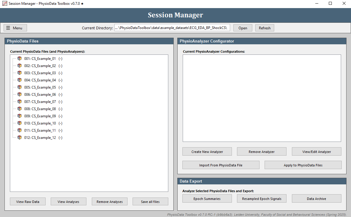
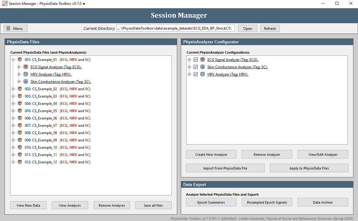
Importing Files
Click on the Open button in the Session Manager and select the folder with the example files (PhysioDataToolbox\data\example_datasets\ECG_EDA_BP_ShockCS\). Alternatively, you can open the example files by going to Menu, selecting Open Example Files and clicking ECG EDA BP ShockCS. The Session Manager should now list all PhysioData files inside the folder (12 in total). Note the PhysioAnalyzers within the files in red. Because we will make new Analyzers in this walkthrough, start by clicking the Remove Analyses button below the file tree, checking all PhysioAnalyzer Tags checkboxes, and clicking the Remove from all files button.
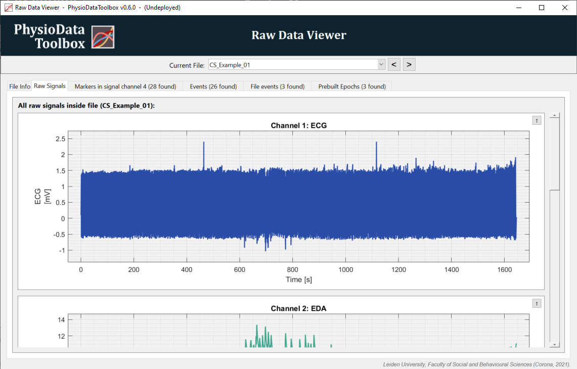
View Raw Data
Click on the View Raw Data button to launch the Raw Data Viewer. The Raw Data Viewer displays all signal channels, events, eye-tracking data, and epochs inside the PhysioData file. When a marker channel is detected, it is automatically analyzed and visualized in a separate tab.
-
Which file is currently being shown is specified in the Current File bar above the tabs. To navigate to a different file, either select it using the dropdown menu, or use the buttons.
-
Click on the Raw Signals tab to see the data. Scroll up and down using the scrollbar to reveal more channels. Take note of what data are in which channel.
To zoom, select a section of the graph using the right mouse button. Double-clicking the graph resets the view. Additional zooming and panning options are available through (a combination of) the other mouse buttons, see the Data Viewers section.
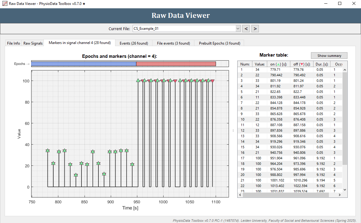
- To view the markers inside the current file, click on the Markers in signal channel 4 tab. In the example files, channel 4 is a digital marker channel, which is automatically detected by the Toolbox.
- Click on the Events tab to see the events inside the current file.

-
Click on the File events tab to view the file events inside the current file.
-
Click on the Prebuilt Epochs tab to view the epochs that were prebuilt in the PhysioData File. Below, in the Defining Epochs chapter we will generate more epochs.
-
When done inspecting the raw data, close the Raw Data Viewer and return to the Session Manager.
Creating PhysioAnalyzer Modules
PhysioAnalyzer modules are signal-specific preprocessing, visualization and analysis pipelines that users can construct and apply to the files. If, for instance, a PhysioData file contains electrocardiogram (ECG) and skin conductance (SC) signals, the user can add ECG and SC modules to the file in order to perform ECG and SC specific analyses on the respective data.
Creating the ECG PhysioAnalyzer
- In the Session Manager, click on the Create New Analyzer button and choose the ECG Signal Analyzer.
- Since ‘ECG’ is a fitting name for the module and the ECG signal is in channel 1 (click the See Channels button to verify this), these settings can be left at their default values.
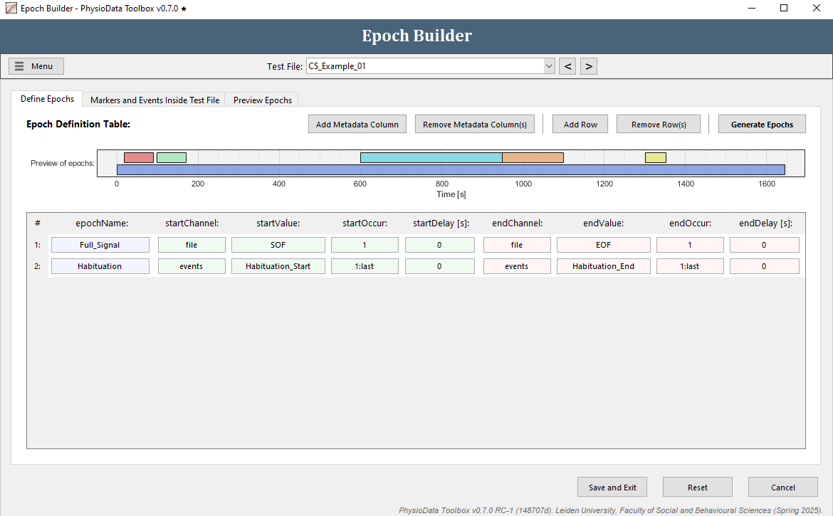
- Click on the View/Edit Epochs button to open the Epoch Builder.
Defining Epochs
Epochs, also called trails or segments, are sections of interest within a recording. Epochs are generally defined relative to markers or events, which are special timestamped moments within the recorded data. The toolbox is designed to automatically segment a signal into epochs using a collection of user-specified rules, and extract relevant metrics for each epoch. For more information on epochs, markers, and events, see the Epochs chapter.
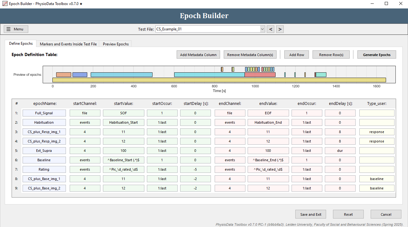
The Define Epochs tab of the Epoch Builder window shows the Epoch Definition Table. Here, the rules for defining epochs are created. By default, an epoch spanning the whole file is created. Notice that in the Preview of epochs graph the prebuilt epochs are also visible.
- Click on the second tab to see all referenceable data inside the current file. In the example files, these are the markers in channel 4, the events, and the file events.
Let’s say we want to create the following epochs:
- Habituation epochs that span from the events ‘Habituation_Start’ to ‘Habituation_End’
- Stimulus epochs:
- CS+ image 1 epochs, that span from the onset of marker with value 11 to 8 seconds later
- CS+ image 2 epochs, that span from the onset of marker with value 12 to 8 seconds later
- Extinction supra epochs that span for the duration of the marker with value 100
NOTE: for more details about the phases of the experiment and their associated markers and events, see the Example Dataset section.
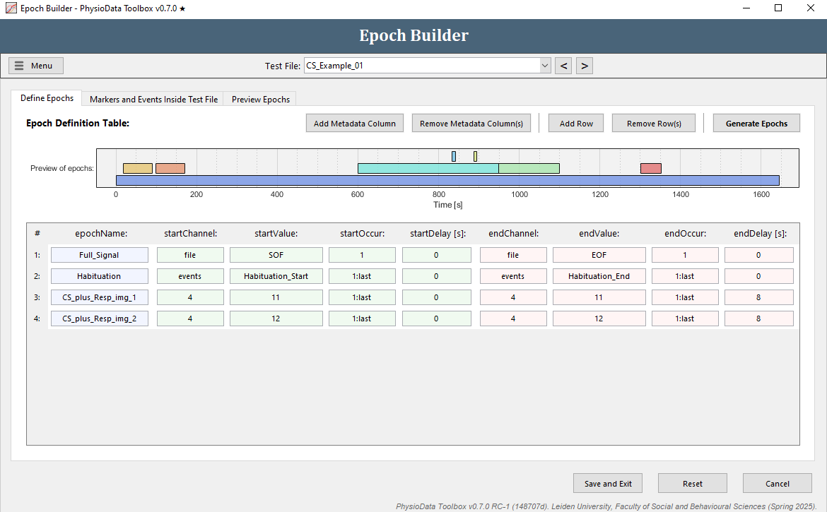
Define the habituation epochs
The epoch definition of the habituation epochs is provided in the Figure below.
- Go back to the Define Epochs tab.
- Click add row.
- In the newly created row, fill in the epochName:
Habituation. - Define the start of the epoch:
- Since we want to reference an event, fill in
eventsin the startChannel field, or right-click on the field and select Channels available in test file and Use Events (26 found). - Fill in the startValue, which is the name of the event, in this case
Habituation_Start(note that the start- and endValue are case-sensitive!), or right-click on the field, select Events available in channel and select Habituation_Start (2 occurrences). - Because we want to create epochs of all habituation segments, we want to reference all ‘Habituation_Start’ events. This is achieved by filling in
1:lastin startOccur, or right-clicking on the field and selecting All occurrences. - The epochs should start directly on the ‘Habituation_Start’ events, therefore we can leave the startDelay at
0.
- Since we want to reference an event, fill in
- Define the end of the epoch:
- The definition of the end of the epoch is pretty similar to the definition of the start of the epoch. We can quickly copy the information of the start of the epoch by right-clicking on any of the end fields, and selecting Copy from start definition.
- Because we want the epoch to end at the ‘Habituation_End’ events, modify the endValue to
Habituation_End, or right-click on the field and select Events available in channel and select Habituation_End (2 occurrences).
- Hit the Generate Epochs button in the top right corner of the tab and observe that two epochs are added in the Preview of epochs graph.
Define the stimulus epochs
The epoch definition of the stimulus epochs is provided in the Figure below.
- Add another row to the Epoch Definition Table.
- In the new row, fill in the epochName:
CS_plus_Resp_img_1. - Define the start of the epochs:
- Since we want to reference markers in channel 4, fill in
4in the startChannel cell (or right-click on the cell and select the appropriate option). Note, the Toolbox will attempt to guess which channel is most likely to be referenced, with preference given to marker channels, when present. As such, in the example dataset,4will be filled in by default when a new row is added. - For the CS+ with image 1 trials, marker 11 was used, fill in
11in startValue (or right-click on the cell and select the appropriate marker). - Because we want to generate epochs from all markers with value 11, fill in
1:lastin startOccur which will take all occurrences (or right-click and select All occurrences). Note that although in file ‘CS_Example_01’ there is only one occurrence of marker 11, this is not the case for other files! - The epochs start at the onset of the marker, therefore the startDelay can be left at
0.
- Since we want to reference markers in channel 4, fill in
- Define the end of the epochs:
- Copy the information of the start of the epoch to the end of the epoch.
- Adjust the endDelay to
8(note that the start- and endDelay are in seconds!).
- Since the CS+ with image 2 epoch definition is very similar to the CS+ image 1 epoch definition, right click on any of the cells of the row we just created and select Duplicate row.
- In the new row, we only need to adjust the epoch name and the marker value to reference the CS+ image 2 trials:
- Fill in
CS_plus_Resp_img_2in epochName. - Fill in
12in startValue and in endValue.
- Fill in
- Hit the Generate Epochs button and check whether the epochs were created correctly.
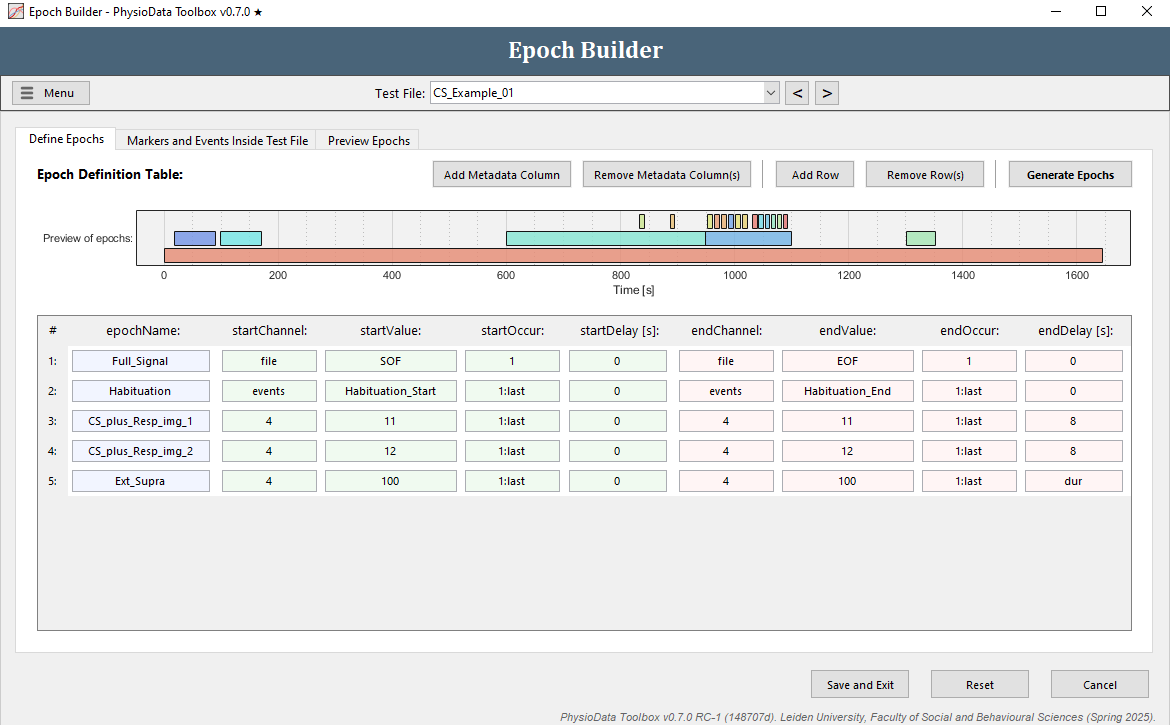
Define the extinction supra epochs
The epoch definition of the extinction supra epochs is provided in the Figure below.
- Add another row.
- Fill in the epochName:
Ext_Supra. - Define the start of the epochs:
- Again, we want to reference markers in channel 4, so make sure the startChannel is set to
4. - Fill in
100in startValue (or right-click on the cell and select the appropriate marker) to reference markers with value 100. - Fill in
1:lastin startOccur to reference all occurrences (or right-click and select All occurrences). - The startDelay can be left at
0.
- Again, we want to reference markers in channel 4, so make sure the startChannel is set to
- Define the end of the epochs:
- Copy the information of the start of the epoch to the end of the epoch.
- Adjust the endDelay to
dur, or right-click on the cell and select Duration of the marker. This will create epochs that span for the duration of the markers (onset to offset).
- Hit the Generate Epochs button and notice that 12 small epochs were created.
Advanced epoch definitions using regular expressions
The following part shows how to create epochs by referencing multiple events with regular expressions. Most users will not need to use them.
Let’s say we also want to create the following epochs:
- Baseline epoch that spans from the event ‘Baseline_Start (<MOVIENAME>)’ to the event ‘Baseline_End (<MOVIENAME>)’.
- Rating epochs that start 5 seconds before the ‘Pic_<ID>_rated_<RATING>’ events and end at the ‘Pic_<ID>_rated_<RATING>’ events.
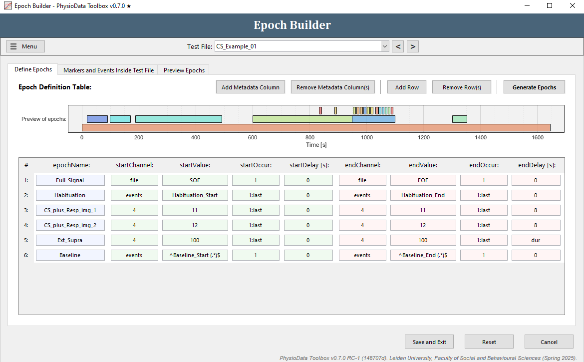
Define the baseline epoch
The epoch definition of the baseline epoch is provided in the Figure below.
- Add another row to the Epoch Definition Table.
- Fill in the epochName:
Baseline. - Define the start of the epoch:
- Fill in
eventsin the startChannel field or right click and navigate to the right channel. - Fill in the startValue. The baseline events start with ‘Baseline_Start’, followed by a space and then the name of the video clip the participant watched in parentheses: ‘Baseline_Start (<MOVIENAME>)’. We can reference all baseline events with all different movie names using one regular expression:
^Baseline_Start (.*)$^and$mark the start and end of the regular expression, respectively..means any single character.*means 0 or more consecutive times.
- Leave startOccur to
1(there is only one baseline segment). - Leave startDelay at
0.
- Fill in
- Define the end of the epoch:
- Copy the information of the start of the epoch to the end of the epoch by right-clicking and selecting Copy from start definition.
- Modify the endValue to
^Baseline_End (.*)$
- Hit the Generate Epochs button and check whether the epoch was created correctly.
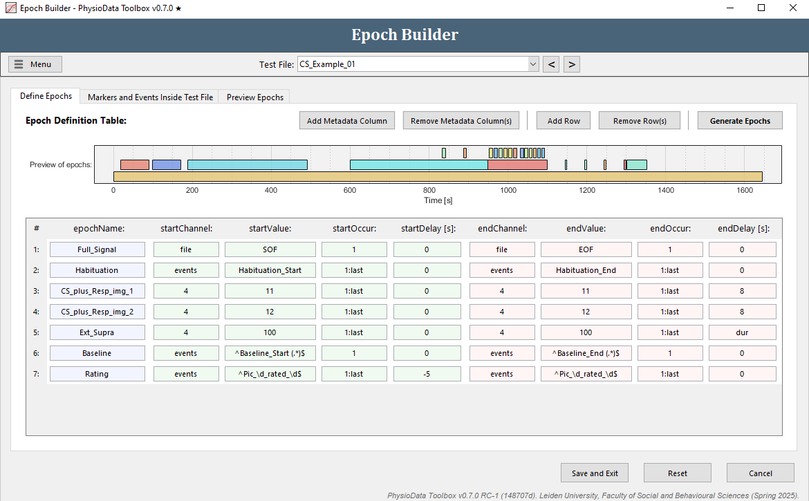
Define the rating epochs
The epoch definition of the rating epochs is provided in the Figure below.
- Click Add Row.
- Fill in the epochName:
Rating. - Define the start of the epochs:
- Fill in
events(or use the right-click option) in startChannel. - We want to reference all the rating events, but because participants gave different ratings to different pictures, the names of these events differ per participant. Again, we can use regular expressions to reference all events with the same pattern. In our case, we want to reference all events with the following pattern: ‘Pic_<ID>_rated_<RATING>’, where <ID> can be a digit ranging 1-4 and <RATING> can be a digit ranging 1-5. In regular expression this translates to
Pic_\d_rated_\d, where\dmeans any numeric digit. When using regular expressions in the Epoch Builder, always start with^and end with$. Thus, fill in^Pic_\d_rated_\d$in startValue. - Reference all occurrences in startOccur.
- We want the epochs to start 5 seconds before the events, therefore, fill in
-5in startDelay.
- Fill in
- Define the end of the epochs:
- Copy the start epoch fields to the end epoch fields.
- We want the epochs to end at the events, therefore fill in
0in endDelay.
- Hit the Generate Epochs button and notice that 4 small epochs were created.
Finish creating the ECG PhysioAnalyzer
When done with creating epochs, click Save and Exit to close the Epoch Builder window and return to the PhysioAnalyzer settings window. We’ll leave the settings to their default values for now (see the ECG Analyzer chapter in the User Guide for more information on the ECG analyzer settings). Click OK to save the changes and return to the Session Manager. Note that although we created an analyzer, the analyzer and the settings and epochs it contains are not applied to the data files yet. We will first create the other analyzers, then apply all analyzers to our data files.
Creating the SC PhysioAnalyzer
- Click the Create New Analyzer button again and select the Skin Conductance Analyzer.
- Fill in
2in the channel number field to make the module use the EDA signal in channel 2. - We will use the same epochs as we defined in the ECG module, therefore, from the drop-down menu to the right of the Generate epochs from label, select PhysioAnalyzer with tag instead of Epoch Definition Table. This will change the View/Edit Epochs button into a text field, into which the tag of the module to be referenced can be entered. As such, fill in
ECGin the field. This will make this module dynamically use any epochs we defined in the ECG module. - Click Ok to close the window and add these settings to the PhysioAnalyzer tree (we’ll leave the settings at their default values, for more information on the Skin Conductance Analyzer settings, see the Skin Conductance Analyzer chapter in the User Guide).
Adding the HRV PhysioAnalyzer
- Click the Create New Analyzer button again and select the HRV Analyzer
- Fill in
ECGin the Tag of the ECG Analyzer field. In order for it to function, the HRV analyzer must be linked to an ECG module. - As with the previous analyzer, we will use the same epochs as we defined in the ECG module. Select PhysioAnalyzer with tag from the epoch drop-down menu and fill in
ECGin the field below. - Click Ok to close the window. We’ll leave the HRV settings to their default, for more information on these settings, consult the HRV Analyzer chapter in the User Guide.
Applying the Settings to the PhysioData files
- In the Session Manager’s PhysioAnalyzer Configurator panel, click the Apply to PhysioData Files and the Apply to all 12 file(s) buttons to propagate the settings of the listed PhysioAnalyzers to all the files. This will create one ECG, one SC, and one HRV module inside each file. Note that the modules inside the PhysioAnalyzer tree on the right side of the Session Manager don’t do anything until they are applied.
- You should now see
ECG, HRV and SCafter each file in the PhysioData file tree. The red color indicates that these modules have not yet been marked as ‘accepted’ by the user. You can expand each file to reveal the PhysioAnalyzers inside it, and each PhysioAnalyzer to reveal its current settings and state. -
Click Remove Analyzer in the PhysioAnalyzer Configurator panel three times to remove the analyzers from this panel. Note that they are still in the files. To reimport the settings from a file, select the desired file and click Import From PhysioData File. This will copy the PhysioAnalyzer settings in that file back to the PhysioAnalyzer Configurator.
Reviewing PhysioAnalyzer Data
This section shows the basics of reviewing and correcting PhysioAnalyzer data.
Launching and Using the PhysioAnalyzer Viewer
- In the Session Manager, click the View Analyses button in the PhysioData Files panel to open the PhysioAnalyzer Viewer window. This window visualizes each PhysioAnalyzer present inside the current file. One tab is created per analyzer.
- The top graph shows the epochs that were generated from the epoch definition. Click on the epochs bar for more epoch information. Below that are the Analyzer-specific data graphs, e.g. for ECG it contains the ECG, Interbeat Interval (IBI) and Instantaneous Heart Rate (IHR) plots. In the legend you can click on a line to hide it. Right-clicking the ECG graph reveals some extra options.
- Inspect the plots inside the ECG and SC tabs using the zooming and panning commands described previously. Use the file bar to navigate through the files.
- Edits made to the current file can be saved by clicking the Save button next to the Menu, as detailed later in this tutorial.
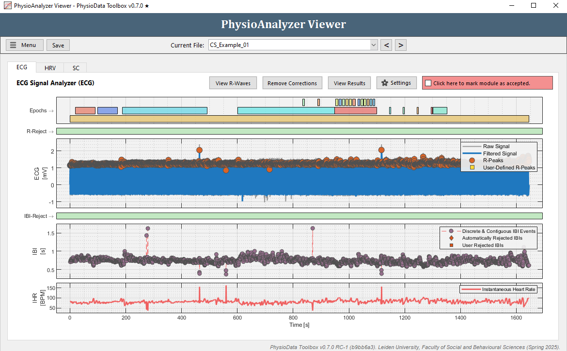
Correcting the ECG data
The ECG module features the ability to mark and reject erroneous R-peaks and IBIs.
- Navigate to the ECG tab in ‘CS_Example_01’.
- Looking at the ECG and IBI plots, a few anomalies can be noticed:
- In the ECG plot there are two R-peaks clearly higher than the other R-peaks at around 500 s and 1100 s. This does not necessarily mean these peaks are faulty, but it is worth checking out.
- In the IBI plot there are a few clear outliers around 300 and 900 s, with high IBI values, and some possible outliers between 400 and 600 s and around 1100 s, with low IBI values.
Note that deviating QRS waves can also be detected by using the View R-Waves button, introduced in version 0.6.2 (info).
-
Zoom in (by selecting an area with the right mouse button) at the high R-peak around 500s. Notice that this peak is not a ‘real’ R-peak, but an extra peak between two R-peaks, resulting in two short IBIs. The R-peak can be removed by selecting an area covering the faulty R-peak (using the left mouse button), and selecting Disable R-Peak detection in the selected section. The disregarded region is visualized in the R-Reject graph above the ECG plot. Notice how removing this R-peak also corrects the faulty IBIs at this time point.

- Zoom in at the 300 s outliers in the IBI plot and notice how this is caused by missing R-waves in the ECG signal, resulting in two instances of doubly long IBIs. This tutorial focusses on how to remove erroneous IBIs. Alternatively, you can manually add missing R-peaks as described here.
-
The IBI artifacts can be manually corrected in a similar manner as removing the R-Peak. Zoom in to the IBI artifact at 274 s, and, using the left mouse button, select an area covering the IBI. Subsequently, select Disregard IBIs in selected section from the menu. The toolbox will now refrain from using any IBIs located inside this newly inserted IBI skip zone, which is visualized in the IBI-skip graph.
Note, to remove an inserted rejection zone, add a new zone the covers the zone you want to remove and select the opposite option. See the Data Viewers page for more information.
-
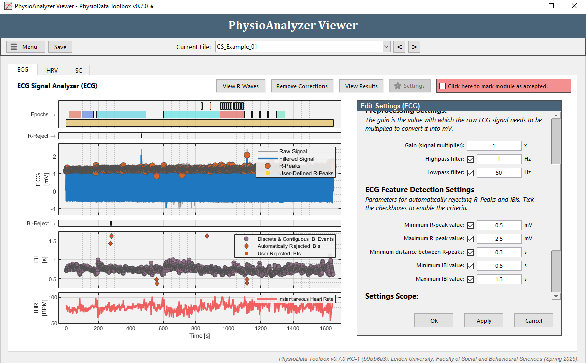
Since manually removing individual IBIs can be time consuming, a better approach may be to adjust the automatic IBI filtering this particular PhysioAnalyzer. Zoom the IBI plot completely out by double clicking it. Notice how the correct IBIs in this file are never located above 1.3 s, or below 0.5 s (zoom in to verify). Click the Settings button in the ECG tab and set the Maximum IBI value to
1.3and the Minimum IBI value to0.5. After clicking Ok, the ECG module will automatically remove all IBIs outside of these thresholds.
In the IBI graph, these automatically rejected IBIs are displayed as diamonds and are not used to generate the Instantaneous Heart Rate (IHR), which is calculated by interpolating all non-rejected IBIs. Note that adjusting the settings within the PhysioAnalyzer Viewer will only affect the current file. Other files are not affected and keep the settings as originally specified when the PhysioAnalyzer was created. Note that only clear outliers can be removed using thresholds. Other erroneous R-peaks and IBIs must be removed manually using rejection zones.
- When done, mark the ECG module in ‘CS_Example_01’ as accepted by clicking the checkbox.
- Press the Save button next to the Menu button to save the corrections you just made in the current PhysioData file.
-
Navigate to the ECG tab in ‘CS_Example_04’ and notice that there seem to be a lot of artifacts in the IBI data.
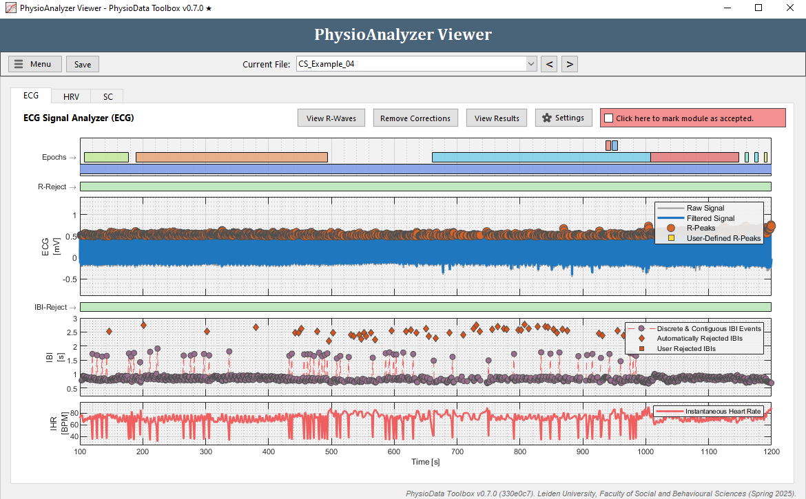
-
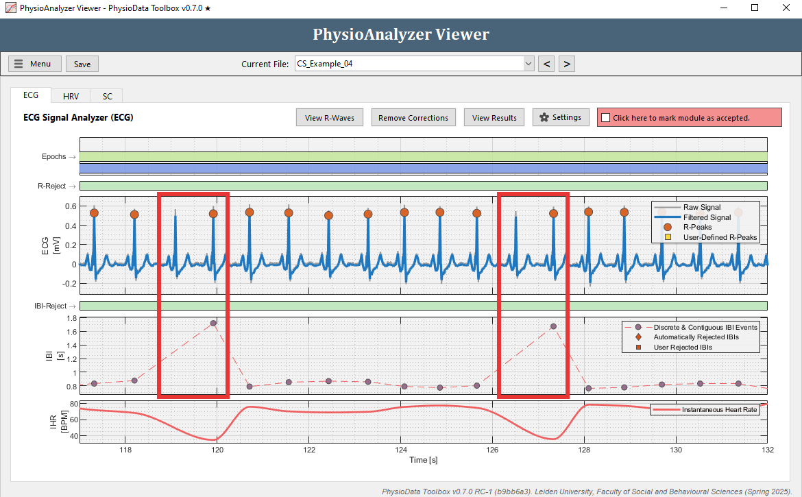
Zoom in at some of the artifacts. Many IBIs are automatically rejected, visualized by diamonds in the IBI graph. Notice that each time before an outlying IBI occurs, an R-peak is ‘missed’ by the PhysioData Toolbox. This means that a ‘true’ R-peak was not detected as R-peak.
- Rather than manually removing each IBI, we can fix this by adjusting the Minimum R-peak value setting in this particular PhysioAnalyzer. Zoom completely out by double clicking on the ECG graph. Notice that the R-peaks hover around 0.5 mV, but do not go below 0.3 mV. Click the Settings button in the ECG tab and set the Minimum R-peak value value to
0.3. After clicking Ok, the ECG module will automatically detect the R-peaks with a value above 0.3.
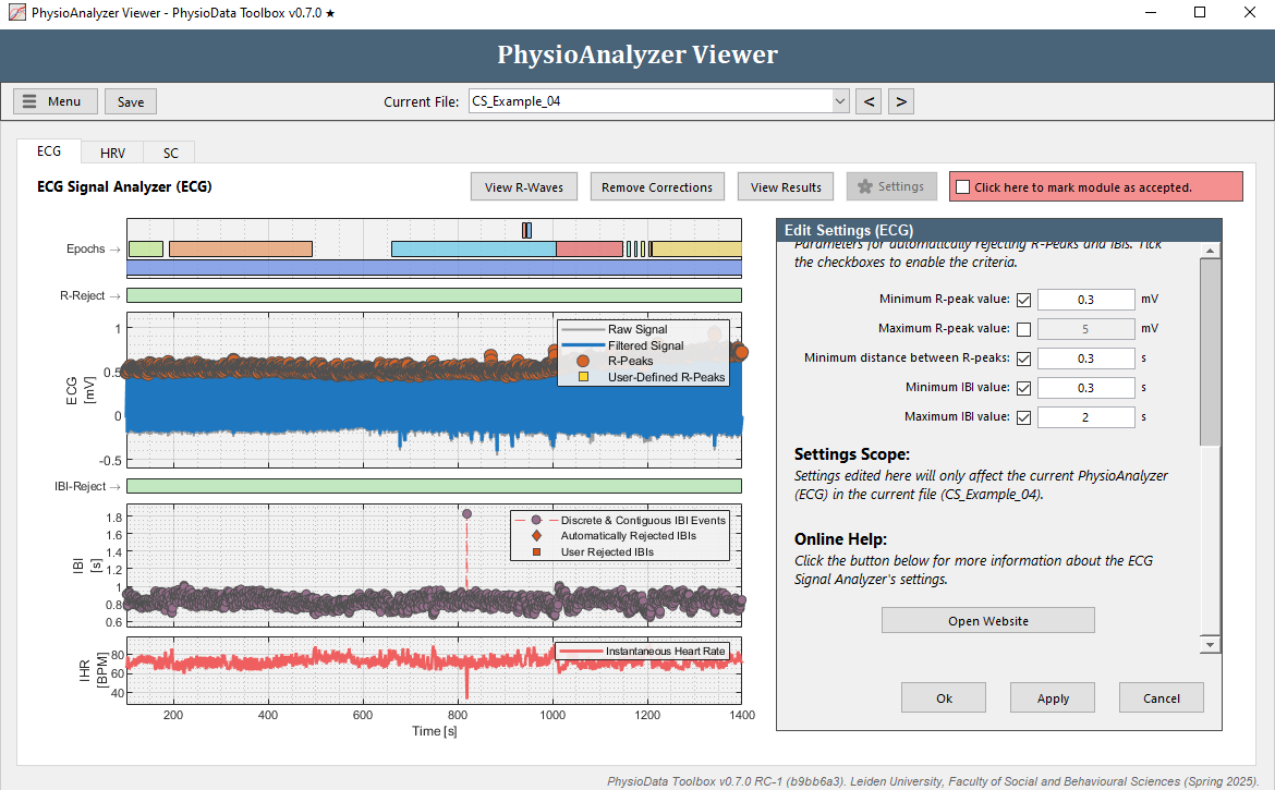
- One outlying IBI remains at around 800 s. Remove this IBI.
- When done, mark this module as accepted by clicking the checkbox.
- Press the Save button to save the corrections in the current PhysioData File.
Correcting the SC data
Data correction in the Skin Conductance graph consists of the user inserting Raw-Skip zones inside which the raw data are not used. Instead, the data inside the zone are replaced by linear interpolation before applying the low-pass filter, and performing the subsequent processing and analysis actions.
- Go the the SC tab in ‘CS_Example_01’. Notice how the skin conductance signal features two downward spikes, possibly caused by the electrodes coming loose (driving down the conductance) and one upwards spike, possibly caused by the electrodes getting short circuited (driving up the conductance).
- In the Skin Conductance graph, zoom in to the artifact at around 650 s. Notice how the (raw) signal is suddenly dropping to 0 and does not reflect any natural skin conductance reaction. However, the toolbox does assign SCR landmarks to this spike (SCR valley and peak). It is thus important to remove these faulty sections.
-
Select a section straddling the artifact. Focus on covering the spike in the gray raw data signal. Select Disregard raw skin conductance data and interpolate to remove the spike. As your not modifying the SCR detection, leave SCR detection on Keep as is.
- Do the same for the other artifacts.
- When done, mark the SC module in ‘CS_Example_01’ as accepted by clicking the checkbox.
- Press the Save button to save the corrections you just made.
Viewing the HRV data
The HRV module itself does not allow users to correct artifacts, this must instead be done in the linked ECG module. Any changes made to the IBIs in the linked ECG module are automatically transmitted to the HRV module, and the graphs and results table are automatically updated. Note that it is important to remove artifacts in both the R-peak and IBI signals in the ECG module. When, for example, the analyzer incorrectly identified an extra R-peak, correcting the corresponding IBI alone will incorrectly mark the preceding and succeeding IBI as noncontiguous, which can have an effect on the HRV results.
-
Navigate to the HRV tab in ‘CS_Example_01’. Note that we previously corrected the IBI signal in the ECG module of this file and that this is also visible when looking at the IBI plot in the top. Zoom in and notice the missing IBIs around 270 s.
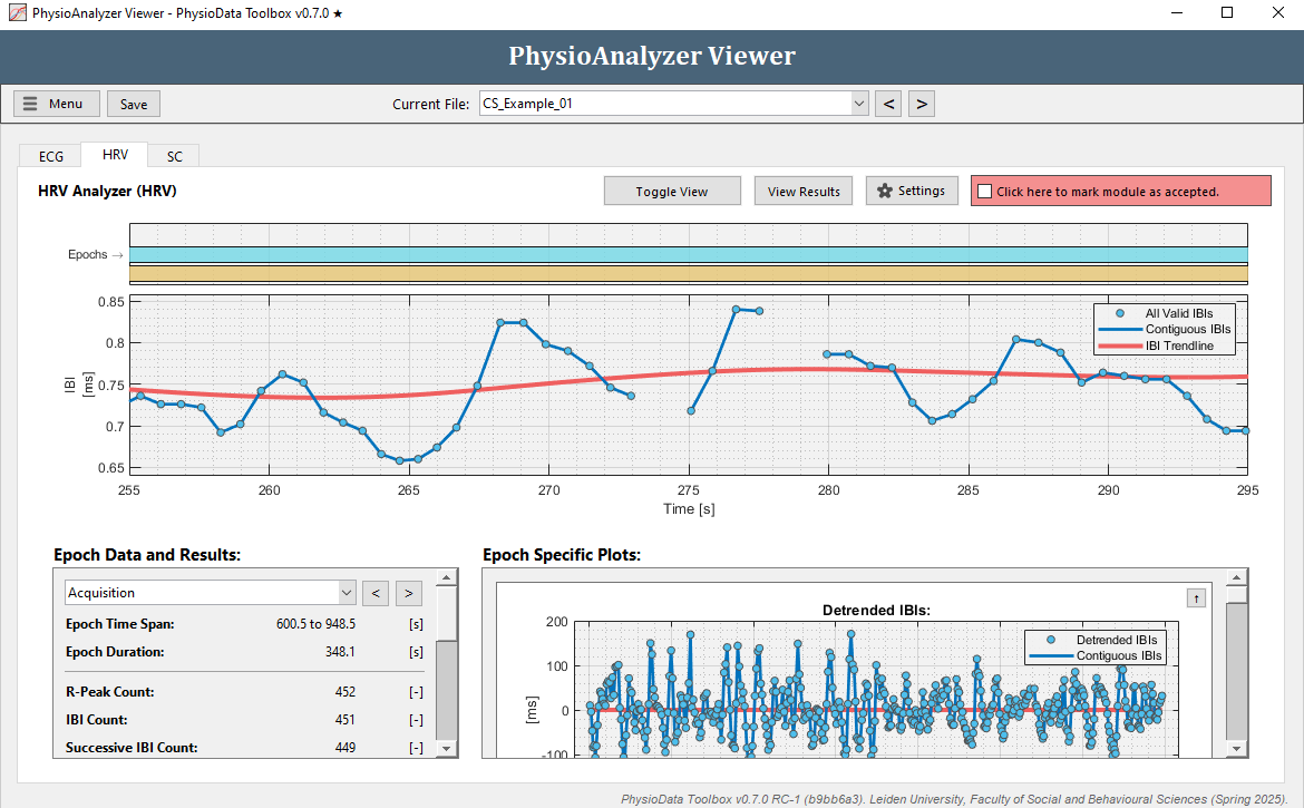
- Select the epoch that you wish to review the results of by using the dropdown menu at the left, or by clicking the buttons next to it, or by clicking on one of the epoch rectangles in the epoch plot in the top of the window.
- Inspect the plots using the zooming and panning commands. In the right bottom part of the window the Detrended IBIs, Successive Differences, Poincare Plot, and Lomb-Scargle Periodogram are displayed. These plots can be minimized by clicking the arrow button in the right upper corner.
- When reviewed, mark the HRV module in ‘CS_Example_01’ as accepted.
Viewing results
- Review the other modules in the other files, correct where necessary, and mark them as accepted.
- You can view each module’s individual results by clicking the View Results button. This will perform descriptive analyses on each epoch in the current PhysioAnalyzer, and show the results in Excel. In the INFO tab summaries of all current settings and states are provided.
- Close the PhysioAnalyzer Viewer when done and go back to the Session Manager.
Updating the Settings
At times it may be necessary to update one or more specific settings within multiple existing PhysioAnalyzers, without overwriting other customized settings, and without removing the corrections. This can be done using the PhysioAnalyzer Configurator in the Session Manager.
Say we want to update the epoch definitions in all files, but leave the other settings intact:
- Select any file in the file tree, and click the Import from PhysioData file button. Remove the Skin Conductance Analyzer and the HRV Analyzer from the PhysioAnalyzer tree by selecting them (by clicking them) and clicking the Remove Analyzer button.
- Click the View/Edit Analyzer button, then in the settings dialog, the Click to View/Edit Epochs button.
- We are going to add trial baseline epochs (ranging 2 seconds before stimulus onset to stimulus onset) that precede the already existing CS+ epochs.
- Add a row.
- Fill in
CS_plus_Base_img_1in epochName. - Leave startChannel at
4. - Fill in
11in startValue. - Fill in
1:lastin startOccur. - Fill in
-2in startDelay. - Copy the start definition fields to the end definition fields.
- Modify the endDelay to
0. - Right click in a field of the row that was just created and select Duplicate row.
- Modify the epochName to
CS_plus_Base_img_2. - Modify the startValue and endValue to
12. - Click Generate Epochs and verify that the epochs were created correctly.
- We will also add a Metadata Column so that more information is included in the exported data:
- Click Add Metadata Column
- Enter
Typein the Column Name field. -
In the newly created column, fill in
responsein ‘Resp’ epochs (rows 3 and 4) andbaselinein the ‘Base’ epochs (rows 8 and 9).
- Click Save and Exit in the Epoch Builder and the Settings dialog to return to the Session Manager.
- Expand the ECG module in the PhysioAnalyzer tree, and deselect all settings except the Epochs (labeled Epochs from definition: 7 row(s) in table).
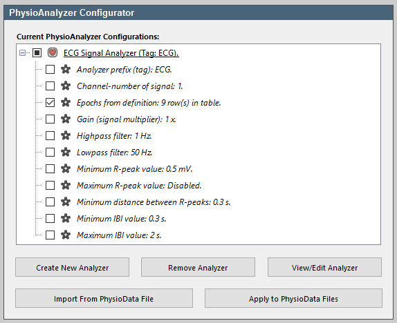
- Click the Apply to PhysioData Files button. This will open a summary of the settings that are to be pushed to the files. Notice that only the epochs are now included in the settings. Click Apply to all files to propagate the listed settings, in this case the epochs, to all the PhysioData files. This will leave the other settings intact. It is also possible to preselect files in the file tree, and push settings only to them.
Note that the Maximum IBI value setting in ‘CS_Example_01’ and the Minimum R-peak value in ‘CS_Examples_04’ were previously customized and differ from the other files. As such, if that setting were not unchecked in the PhysioAnalyzer tree, its value would be pushed to all files overwriting any file-specific values.
- Use the PhysioAnalyzer viewer to verify that the new epochs are present in all files, and that the customized Maximum IBI value setting in ‘CS_Example_01’ and Minimum R-peak value in ‘CS_Examples_04’ are still intact.
Exporting Analysis
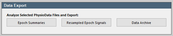
The results of all the PhysioAnalyzers inside multiple PhysioData files can be exported to different file formats, by first selecting the desired PhysioData files in the file tree, then clicking the Epoch Summaries button in the Data Export panel. We will export the data to an Excel file.
- Select all PhysioData files (tip: use ctrl + A).
- Click the Epoch Summaries button, then click Analyze all files, wait for the toolbox to collect the descriptive analyses and then select As one Excel file, with one table per worksheet and click Ok. Finally, click the Open Excel File button to view the file. The results are automatically saved to a new timestamped Excel file in the current data directory.
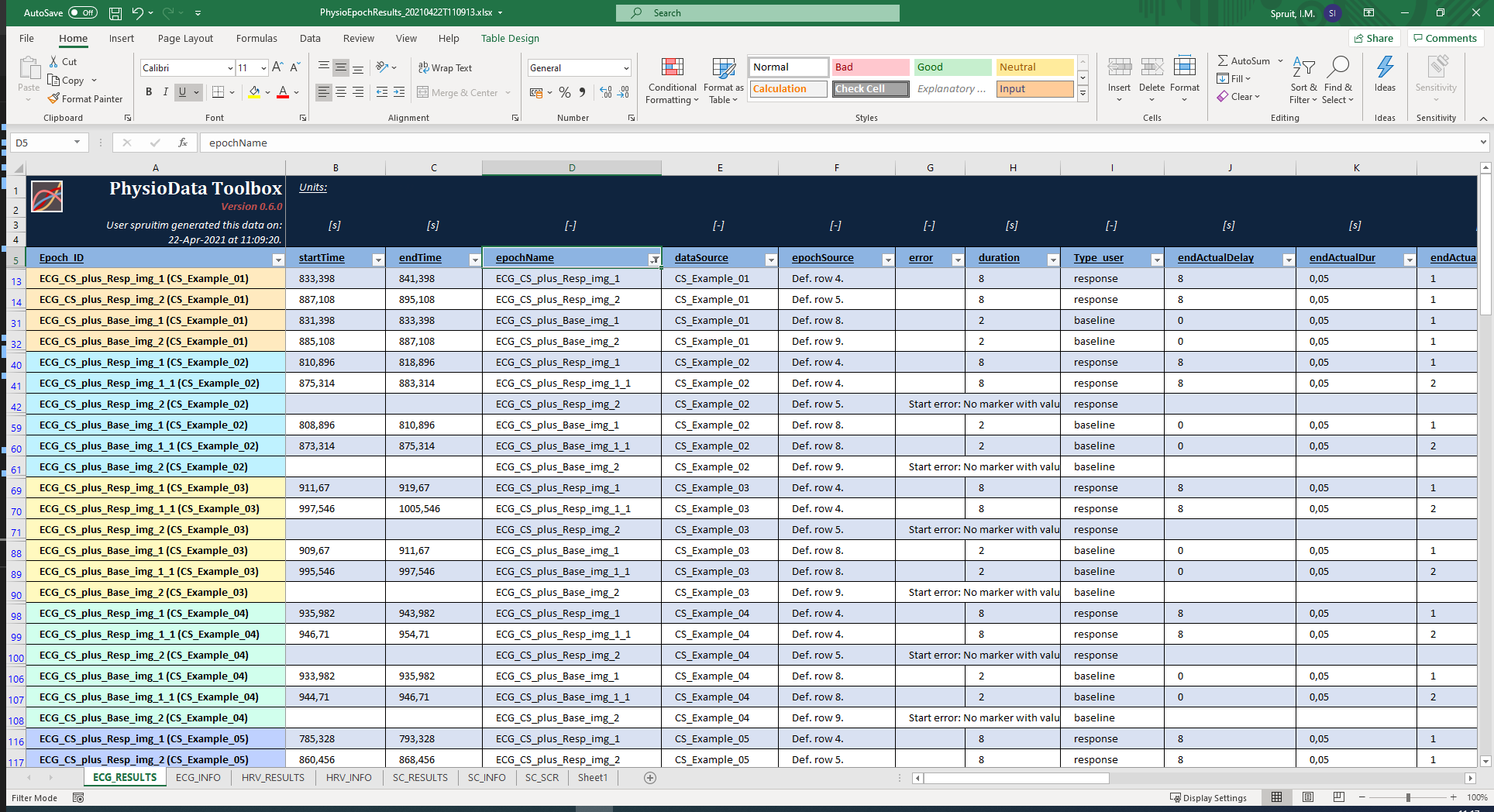
- For each unique PhysioAnalyzer tag, two new sheets are created: the <tag>_RESULTS and <tag>_INFO sheets. These sheets can be accessed using the tabs in the bottom left corner of the Excel window. The ‘RESULTS’ sheet contains all the results for all epochs in that PhysioAnalyzer, inside all selected files. Notice that these results include the user created Metadata column Type_user. The ‘INFO’ sheet contains information about the settings and state. Rows that belong to the same file are grouped together by color in the first column.
- Note that the data are automatically formatted as Excel tables, allowing you to easily filter and sort the data. As an example, the table can be filtered to only show the stimulus baseline and response epochs by clicking the button in the epochName table header (cell D:5), and selecting only the stimulus epochs (that start with ‘ECG_CS’).
Saving the session
Edits made to PhysioData files can be saved in individual files by clicking the Save button in the PhysioAnalyzer Viewer. This will save the PhysioAnalyzers, including their settings and state, and all user corrections in that PhysioData file. To save all files, click the Save all files button in the Session Manager.
It is strongly advised to save often to prevent data loss in case the PhysioData Toolbox inadvertently closes.
Note, only PhysioAnalyzers that have been applied to PhysioData files are saved inside their respective files. Those PhysioAnalyzers are visualized in the file tree inside the PhysioData files panel in the Session Manager. PhysioAnalyzers in the PhysioAnalyzer configurator are not saved and will be lost when the Toolbox is closed.